Machine learning: XGBoost vs. Random forests
Published:
Please note this page is under active development
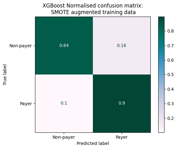
In this page, I continue exploring ML methods to predict loan payback. The code below is a follow up to the the logistic regression approach used as baseline in the previous page. What I seek to explore here is whether other supervised methods can deliver better performing methods, with a focus on reducing the false positive rate seen in logistic regression (i.e., reducing then umber of non-payers incorrectly classified as payers).
I’ll be using scikit-learn along other packages shown below. The specific environment used for the entire project is available here.
# set up
import pandas as pd
import matplotlib.pyplot as plt
import numpy as np
# ml methods
from sklearn.model_selection import train_test_split, cross_validate, \
    cross_val_predict, StratifiedKFold, KFold
from sklearn.linear_model import LogisticRegression
from sklearn.ensemble import RandomForestClassifier
from sklearn.preprocessing import StandardScaler
# new?
from sklearn.ensemble import VotingClassifier
from sklearn.metrics import RocCurveDisplay, confusion_matrix,\
    ConfusionMatrixDisplay, classification_report
from xgboost import XGBClassifier
Use SMOTE augmented data:
- data upload
- data splitting
data_encoded_smote = pd.read_csv('./data/data_processed_after_smote.csv')
data_augmented = data_encoded_smote.copy()
data_augmented = data_augmented.drop(columns=['is_synthetic',
                                        'nearest_neighbour_distance',
                                        'nearest_neighbour_index_real_data'])
# separate features and labels (outcome)
X = data_augmented.drop('loan_paid_back', axis=1)
y = data_augmented['loan_paid_back']

# data splits: training, validation, and testing
# (80% for training/validation, 20% for testing)
X_train, X_test, y_train, y_test = train_test_split(X, y, test_size=0.2,
                                                    random_state=17)
Functions for modelling pipeline
Develop functions to set a training pipeline. Note features won’t be standardsised (as done in logistic regression), as we’re using tree-based ML methods.
# cross validation results for a tree-based model
def cross_validate_results(
              name="XGBoost",
              model=XGBClassifier(random_state=42),
              X_train=X_train,
              y_train=y_train,
              ):

    # use stratified cross validation (cv) - i.e., percentage of sample
    # in each label is kept consistent as possible
    cv_results = cross_validate(
        model, X_train, y_train,
        # performance metrics to calculate
        scoring=['accuracy', 'precision', 'recall', 'f1'],
        n_jobs=-1,
        # number of folds
        cv=10,
        )

    results = pd.DataFrame(cv_results)

    # use model name as index for results dataframe
    results['model_name'] = name
    results.set_index('model_name', inplace=True)

    return results

# plot performance metrics from cross validation results
def plot_performance_metrics(cv_results, name):
    # plot distribution of performance metrics shown in classification report
    performance_metrics = pd.DataFrame(cv_results).drop(
        columns=['fit_time', 'score_time'])

    # plot metrics obtained via stratified kfolds
    # the test_ metrics refer to the the 10th fold
    plt.subplots(figsize=(8,5))
    plt.boxplot(performance_metrics, labels=performance_metrics.columns)
    plt.ylabel('Score')
    plt.tight_layout()
    plt.title(f"{name} Performance metrics from 10-fold cross validation")
    plt.show()

# plot confusion matrix
def plot_confusion_matrix(fitted_model, name):
    ConfusionMatrixDisplay.from_estimator(fitted_model, X_train, y_train,
                                        display_labels=['Non-payer','Payer'],
                                        cmap='PuBuGn',
                                        normalize='true'
                                        )
    plt.title(f'{name} Normalised confusion matrix:\n SMOTE augmented training data')
    plt.show()

# plot receiver operator characteristic curve
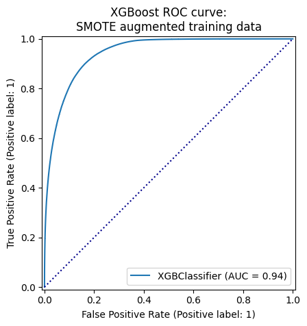
def plot_roc_curve(fitted_model, name):
    # receiver operator characteristic curve
    # plot specificity (false positive rate) vs recall (aka sensitivity; true positive rate)
    roc_curve = RocCurveDisplay.from_estimator(fitted_model, X_train, y_train, pos_label=1)
    fig = roc_curve.figure_
    ax = roc_curve.ax_
    # plot chance
    ax.plot([0,1], [0,1], color='darkblue', linestyle=':')
    plt.title(f'{name} ROC curve:\nSMOTE augmented training data')
    plt.show()
Model comparisons
# define models to compare
model_random_forest = RandomForestClassifier(random_state=42)
model_xgb = XGBClassifier(random_state=42)
# compare performance metrics
results_xgb = cross_validate_results(model = model_xgb, name = "XGBoost")
results_random_forest = cross_validate_results(model = model_random_forest, name = "Random Forest")
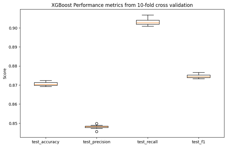
plot_performance_metrics(results_xgb, name="XGBoost")
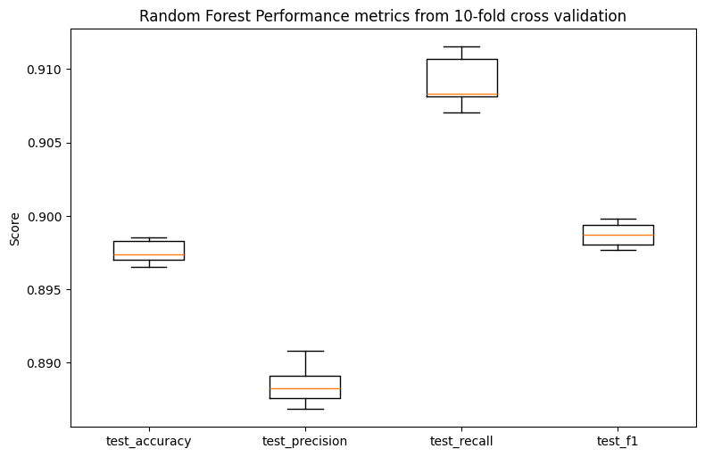
plot_performance_metrics(results_random_forest, name="Random Forest")
# fit models and plot confusion matrices
model = model_xgb
model.fit(X_train, y_train)
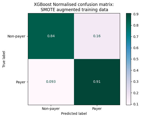
plot_confusion_matrix(model, name="XGBoost")
# plot receiver operator characteristic curves
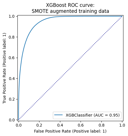
plot_roc_curve(model, name="XGBoost")
# fit models and plot confusion matrices
model = model_random_forest
model.fit(X_train, y_train)
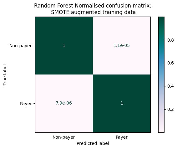
plot_confusion_matrix(model, name="Random Forest")
# plot receiver operator characteristic curves
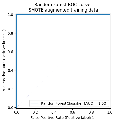
plot_roc_curve(model, name="Random Forest")
Conclusions
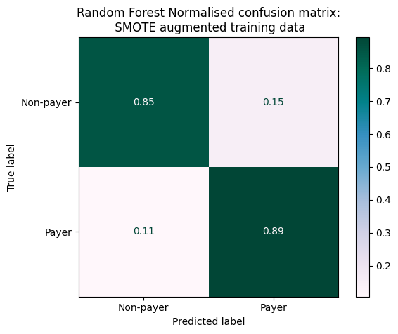
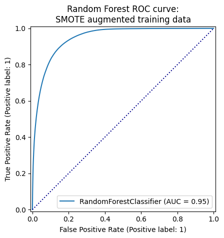
- Random forest results in better performance metrics, but this method is known to overfit data. The very small proportions of incorrect predictions could be interpreted as a sign of overfitting and ROC curve suggests our random forest was a perfect classifier.
- Evaluating the
# evaluate using test data
model = model_xgb
model.fit(X_test, y_test)
plot_confusion_matrix(model, name="XGBoost")
# plot receiver operator characteristic curves
plot_roc_curve(model, name="XGBoost")
# evaluate using test data
model = model_random_forest
model.fit(X_test, y_test)
plot_confusion_matrix(model, name="Random Forest")
# plot receiver operator characteristic curves
plot_roc_curve(model, name="Random Forest")